Calculating Doppler Spread from WSPR Data

November 1, 2023 2 minutes read

Purpose

After examining the Doppler spread (w50) algorithm from FST4 and trying to understand how wpsrd works I decided to take the plunge and see if I could calculate Doppler spread from WSPR data. My initial idea was to use the c2 files created by wsprd as a data source. Thanks to the wsjtx-devel list, I soon discovered c2 files didn’t have the data I thought they did.

So what I ended up implementing is a Python program that takes a WAV file as well as the wsprd output and calculates the Doppler spread for each decoded signal. In the process of testing the Python program I ended up with a patch for wsprd.c as well. You can find them both here.

wspr.py

While wsprd has all sorts of functions available to it for doing things like generating a reference signal as required by the Doppler spread algorithm, I didn’t have much available for me in Python. That’s not to say that WSPR encoding is not well documented, it’s far better documented than WSPR decoding, but my options in Python were not as easy-to-use and well documented as I wished.

As such, I wrote a Python implementation. I’ll quote directly from its module docstring here (remember I said I was aiming for well documented):

This module implements functions required to encode WSPR messages. It is largely based on the G4JNT’s excellent reference: http://www.g4jnt.com/wspr_coding_process.pdf as well as SM0YSR’s wspr-tools: https://github.com/robertostling/wspr-tools" The goal was to make an easy-to-understand, well-documented Python WSPR encoder implementation.

Feel free to yank this file out and do whatever you like with it. It currently only supports simple, two minute transmissions, but for my purposes of generating a symbols array it works great.

wspr_spread.py

Let’s jump into the internals of the program to understand how it works and what its limitations are.

Reading the WAV file

There are a couple of different ways I can approach calculating the Doppler spread with WAV data:

I could take the samples straight from the WAV file (two minutes at 12,000 samples/sec), generate a reference waveform with the same number samples and calculate g(t) by multiplying the raw data by the complex conjugate of the reference waveform.
I could process the WAV file the same way wsprd.c does, downsampling it and working it into complex IQ data with 46080 samples.

I chose the second option as I suspected this work would be best done inside wsprd.c and at some point I intended to create and submit a patch. While the second option may not be the fastest for a pure Python implementation, it should demonstrate how much of the work that wsprd.c does is replicated and make it easier to write the patch.

If you take a look a read_wav_file() in wspr_spread.py it’s almost taken exactly from readwavfile() in wsprd.c. It does a bit more WAV file error checking as I had the whole wave Python package at my disposal, so why not. It performs a forward and reverse FFT via numpy.fft to resample and isolate a 375 Hz subsection. Some attention must be paid to the normalization as FFTW and numpy.fft are slightly different. Finally it returns a complex numpy array as opposed to idat and qdat arrays. This function was checked by analyzing the output and making sure it matched with the wsprd.c readwavefile() results.

Reading the wsprd output

read_wsprd() reads an ALL_WSPR.txt format file, which looks something like this:

sprd mple  -9  1.13   0.0014463  ND6P DM04 30            0  0.68  1  1    0  0   0     1   612
sprd mple -15  0.07   0.0014604  W5BIT EL09 17           0  0.48  1  1    0  0   7     1   500
sprd mple -23  2.16   0.0014652  G8VDQ IO91 37           0  0.22  3  1   16  0   0  8080  -187
sprd mple  -6  0.62   0.0014891  WD4LHT EL89 30          0  0.66  1  1    0  0   2     1   539
sprd mple  -1 -0.79   0.0015028  NM7J DM26 30            0  0.33  1  1    0  0  26     1    45
sprd mple -21  0.54   0.0015174  KI7CI DM09 37           0  0.36  1  1    0  0   3     1   557
sprd mple -18 -1.94   0.0015298  DJ6OL JO52 37           0  0.35  1  1    0  0  11     1   364
sprd mple -11  0.83   0.0015868  W3HH EL89 30            0  0.73  1  1    0  0   0     1   734
sprd mple -25  0.75   0.0015944  W3BI FN20 30            0  0.14  2  1    0  0  30  1223   -90

It transforms it into a Python dictionary to make it easy to get the data we need to generate the reference signal. Using this file instead of the output of the wsprd program gives us 0.1 Hz accuracy in the reported frequency.

You may also notice that the date is listed as sprd and time is listed as mple. That’s because the time is automatically derived from the filename.

Usage

usage: wspr_spread.py [-h] [-d] wav_file all_wspr

Calculates the Doppler spread (w50) of signals decoded by wsprd

positional arguments:
  wav_file     WAV file of WSPR audio (same format was wsprd)
  all_wspr     ALL_WSPR.txt format file with wsprd output (defaults to ALL_WSPR.txt)

optional arguments:
  -h, --help   show this help message and exit
  -d, --debug  Print debugging messages and create FFT graphs

Usage is pretty basic, it only needs information about the decoded signals (to build a reference signal) and a WAV file of the signal. You can see the sample ALL_WSPR.txt file and it’s corresponding WAV file, sample.wav, in the source directory.

Results

Initially the results weren’t great, at least for the sample that I’ve was working with. They caused me to check and re-check my Python code to see if it actually makes sense. This delayed me for months.

I actually ended up implementing a wsprd.c patch, which I was planning to do later, just to see if it had better results. I defined a calc_g() function to attempt to mimic that way wsprd.c computes it’s c(t) leaving some space at the beginning of the array. By carefully working on wspr_spready.py and wsprd.c I was able to get some better results out of wspr_spread.py. For more detail on the limitations and details see A wsprd.c Patch.

If you enable the debug option, wspr_spread.py will use matplotlib to create several graphs to try and show what’s going on. Let’s take a look at a few.

First of all, here’s the output for my sample. The last column is Doppler spread:

$ python3 wspr_spread.py sample.wav ALL_WSPR.TXT
  sprd mple  -9  1.13   0.0014463  ND6P DM04 30            0  0.68  1  1    0  0   0     1   612  0.171
  sprd mple -15  0.07   0.0014604  W5BIT EL09 17           0  0.48  1  1    0  0   7     1   500  0.374
  sprd mple -23  2.16   0.0014652  G8VDQ IO91 37           0  0.22  3  1   16  0   0  8080  -187  0.781
  sprd mple  -6  0.62   0.0014891  WD4LHT EL89 30          0  0.66  1  1    0  0   2     1   539  0.203
  sprd mple  -1 -0.79   0.0015028  NM7J DM26 30            0  0.33  1  1    0  0  26     1    45  0.545
  sprd mple -21  0.54   0.0015174  KI7CI DM09 37           0  0.36  1  1    0  0   3     1   557  0.081
  sprd mple -18 -1.94   0.0015298  DJ6OL JO52 37           0  0.35  1  1    0  0  11     1   364  0.472
  sprd mple -11  0.83   0.0015868  W3HH EL89 30            0  0.73  1  1    0  0   0     1   734  0.041
  sprd mple -25  0.75   0.0015944  W3BI FN20 30            0  0.14  2  1    0  0  30  1223   -90  0.545

The FFT of the IQ data looks like this:

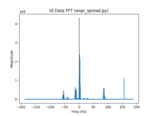
As expected from the decoding information, we see a large signal close to 0 Hz offset, NM7J, and various other signals. I’ll start by taking a look at the NM7J signal. Here’s the FFT of a reference signal generated for the NM7J signal’s message and frequency:

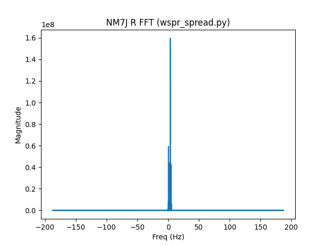
It’s centered around 3 Hz and occupies about 4 Hz of bandwidth. You can’t tell from the FFT, but in the time domain it’s scaled between -1 and 1.

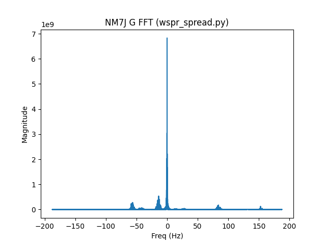
So far so good, let’s multiply our IQ data by the complex conjugate of our reference signal to get the estimated channel gain data (g). Here’s an FFT of g for the NM7J signal:

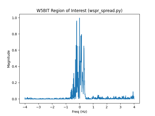
Now let’s take a look at the region of interest (-4 Hz to 4 Hz of g) after we’ve scaled it an subtracted out the noise:

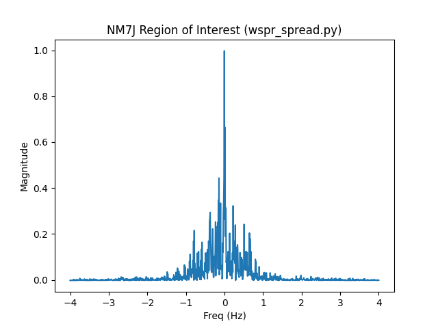
That looks OK to me, centered on a signal with the power region between -1 and 1 Hz. It’s certainly not as tight was what my FST4 sample was, but I don’t know if that’s due to the sample, protocol, or anything else.

The Doppler spread (w50, the bandwidth over which 50% of the power of the signal exists) ends up being 0.545 when you calculate it.

Let’s take a look at the region of interest for the signal with the lowest Doppler spread, W3HH:

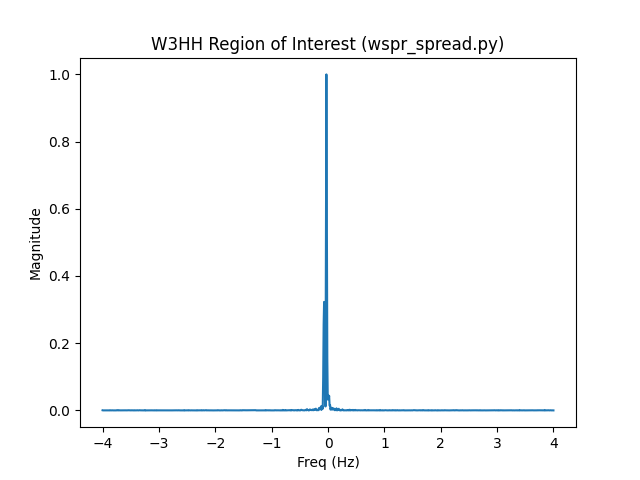
That looks more comparable to my FST4 sample. Sure enough when calculated it has a tight Doppler spread of 0.041.

A wsprd.c Patch

In the process of trying to get wsprd_spread.py to work I ended up spending a lot of time modifying wsprd.c. By the time I was done, I had most of a wsprd.c patch for calculating Doppler spread implemented.

wsprd.c does parts of the Doppler spread calculation in its subtract_signal2() function as part of removing signals.^[1] Here’s a comment from that code:

    /******************************************************************************
     Measured signal:                    s(t)=a(t)*exp( j*theta(t) )
     Reference is:                       r(t) = exp( j*phi(t) )
     Complex amplitude is estimated as:  c(t)=LPF[s(t)*conjugate(r(t))]
     so c(t) has phase angle theta-phi
     Multiply r(t) by c(t) and subtract from s(t), i.e. s'(t)=s(t)-c(t)r(t)
     *******************************************************************************/

Using their terminology we want c(t) which corresponds to our g (estimated channel gain data). This patch adds Doppler spread data to the ALL_WSPR.txt output: I implemented a dopsread() function which uses the c(t) calculated as part of wsprd.c:

/******************************************************************************
  Calculate the doppler spread (w50) from g (estimated channel gain data, c(t))
 *******************************************************************************/
float dopspread(float *ci, float *cq)
{
    int i, j;
    int nsym = 162;
    int nspersym = 256;
    int points = nsym * nspersym;
    fftwf_plan plan;
    fftwf_complex *g, *g_fft;
    float *roi;
    float df = 375.0/points;
    float max_power = 0, total_power = 0, curr_power = 0;
    int roi_points = 0;
    int right_noise_points = 0;
    int left_noise_points = 0;
    float left_noise = 0, right_noise = 0, noise, freq;
    int i25 = 0, i75 = 0;
    float doppler_spread;

    /* take an FFT of c(t) from subtract_signal2() */
    g = (fftwf_complex*) fftwf_malloc(sizeof(fftwf_complex) * points);
    for (i = 0; i < points; i++) {
	g[i][0] = ci[i];
	g[i][1] = cq[i];
    }
    g_fft = (fftwf_complex*) fftwf_malloc(sizeof(fftwf_complex) * points);
    plan = fftwf_plan_dft_1d(points, g, g_fft, FFTW_FORWARD, PATIENCE);
    fftwf_execute(plan);

    for (i = (-187.5 / df); i < (187.5 / df); i++) {
	j = i;
	if (j < 0) {
	    j = i + points;
	}
    }

    /* pull out the region of interest (-4 to 4 Hz), shift the zero freq
     * component to the center of the array, convert to power, and find the
     * maximum power between -1 and 1 Hz */
    roi = fftwf_malloc(sizeof(float) * ((8.0 / df) + 0.5));
    roi_points = 0;
    for (i = (-4.0 / df); i < (4.0 / df); i++) {
	j = i;
	if (j < 0) {
	    j = i + points;
	}
    	roi[roi_points] = (g_fft[j][0] * g_fft[j][0]) + (g_fft[j][1] * g_fft[j][1]);
	if ((i > (-1.0 / df)) && (i < 1.0 / df)) {
	    if (roi[roi_points] > max_power) {
	        max_power = roi[roi_points];
	    }
        }
    	roi_points++;
    }

    /* scale the region of interest by the max power and find the average
     * noise in the -4 and -2 Hz and 2 and 4 Hz regions */
    for (i = 0; i < roi_points; i++) {
	roi[i] = roi[i] / max_power;
	freq = (i * df) - 4;
	if ((freq > -4.0) && (freq < -2.0)) {
	    left_noise = left_noise + roi[i];
	    left_noise_points++;
	} else if ((freq > 2.0) && (freq < 4.0)) {
	    right_noise = right_noise + roi[i];
	    right_noise_points++;
	}
    }
    left_noise = left_noise / left_noise_points;
    right_noise = right_noise / right_noise_points;

    /* subtract out the noise using whichever noise side is lower and calculate
     * the total power between -1 and 1 Hz */
    noise = (left_noise > right_noise) ? right_noise : left_noise;
    for (i = 0; i < roi_points; i++) {
	roi[i] = roi[i] - noise;
	freq = (i * df) - 4;
	if ((freq > -1.0) && (freq < 1.0)) {
	    total_power += roi[i];
	}
    }

    /* find the indexes where the power reaches 25% of the total and 75% */
    for (i = ((-1 + 4) / df); i < ((1 + 4) / df); i++) {
	curr_power += roi[i];
	if (((curr_power / total_power) > 0.25) && (i25 == 0)) {
	    i25 = i;
	}
	if (((curr_power / total_power) > 0.75) && (i75 == 0)) {
	    i75 = i;
	}
    }

    /* Doppler spread is the frequency difference between those points */
    doppler_spread = (i75 - i25) * df;

    fftwf_destroy_plan(plan);
    fftwf_free(g);
    fftwf_free(g_fft);
    fftwf_free(roi);

    return doppler_spread;
}

Here’s the ALL_WSPR.txt output I get when I run the patched wsprd on my sample. Doppler spread is the last column.

sprd mple  -9  1.13   0.0014463  ND6P DM04 30            0  0.68  1  1    0  0   0     1   612  0.145
sprd mple -15  0.07   0.0014604  W5BIT EL09 17           0  0.48  1  1    0  0   7     1   500  0.127
sprd mple -23  2.16   0.0014652  G8VDQ IO91 37           0  0.22  3  1   16  0  35  8080  -187  0.515
sprd mple  -6  0.62   0.0014891  WD4LHT EL89 30          0  0.66  1  1    0  0   2     1   539  0.199
sprd mple  -1 -0.79   0.0015028  NM7J DM26 30            0  0.33  1  1    0  0  26     1    45  0.570
sprd mple -21  0.54   0.0015174  KI7CI DM09 37           0  0.36  1  1    0  0   3     1   557  0.081
sprd mple -18 -1.94   0.0015298  DJ6OL JO52 37           0  0.35  1  1    0  0  11     1   364  0.443
sprd mple -11  0.83   0.0015868  W3HH EL89 30            0  0.73  1  1    0  0   0     1   734  0.009
sprd mple -25  0.75   0.0015944  W3BI FN20 30            0  0.14  2  1    0  0  30  1223   -90  0.488

You’ll notice some big Doppler spread differences between what wspr_spread.py and the patched wsprd calculates. Here’s a side-by-side comparison:

Table 1. Dopppler Spread Differences Between Implementations
Callsign	Patched wsprd	wspr_spread.py	% difference
ND6P	0.145	0.171	16
W5BIT	0.127	0.374	99
G8VDQ	0.515	0.781	41
WD4LHT	0.199	0.203	2
NM7J	0.570	0.545	5
KI7CI	0.081	0.081	0
DJ6OL	0.443	0.472	6
W3HH	0.009	0.041	128
W3BI	0.488	0.545	11

This begs the question, what’s going on with the W3HH and W5BIT signals? Let’s pull the regions of interest out of dopspread() in wsprd.c and compare them with the regions of interest from wspr_spread.py:

They look similar, but noticeably different. This lead me down a rabbit hole of comparisons and debugging output that ate up even more time. I’ll save you the pain and just summarize with a list of reasons wsprd.c and wspr_spread.py yield very different results for some signals:

wsprd.c has access to more accurate frequency and time shift data. 0.1 Hz and 0.01 second resolution when reading from an ALL_WSPR.txt file does not yield great results.
wsprd.c uses a tone spacing of 1.5 instead of 12000 / 8192.
Because dopspread() is called from subtract_signal2(), wsprd.c will calculate the Doppler spread using IQ data that may have already had strong signals subtracted from it. In my testing this doesn’t seem to make a huge difference, but it’s certainly something to keep in mind.
wsprd.c will also calculate Doppler spread for signals who’s frequency drifts over time. This may not actually be a big deal as the reference signal is generated to follow the frequency shift (linearly) over time so the FFT of the resulting g should represent the actual signal. It’s worth noting that none of my testing samples had frequency drifts.
wsprd.c uses single precision (32 bit) floats while wspr_spread.py uses double precision floats (64 bits). This actually accounts for the majority of the difference you see (think W3HH and W5BIT). While it may seem inconsequential, the precision difference when generating a reference signal is compounded forty thousand times. You can make wsprd_spread.py get even closer to wsprd.c output (0.02 for the spread of the W3HH signal) if you judiciously use Numpy’s float32 type. It takes a lot of effort and it’s technically less accurate.

Conclusion

Pick one way of calculating Doppler spread from WSPR data and stick to it. The reasons you get different results are subtle and hard to debug. Some reasons lend themselves to making the wspr_spread.py result more accurate and others make wsprd.c more accurate.

If you were really ambitious, you could rewrite wsprd.c to use double precision floats (constants in C are already double precision, you could use the default FFTW options). Likewise you could use 12000 / 8192 tone spacing in subtract_signal2(). Based on what I’ve seen, I don’t think it will make that much of a difference in wsprd’s ability to decode signals, and ultimately that’s the primary thing that wsprd does.

1. This will only calculate Doppler spread when subtraction is enabled in wsprd!