FST4 Doppler Spread Algorithm in WSJT-X

I used the WSJT-X CMake script to clone the latest version of the modified hamlib and wsjtx and confirmed that I could compile everything. This was basically a matter of following the steps in the INSTALL file. I then downloaded 60 second FTS4 signal (210115_0058.wav) and confirmed that I could use the jt9 utility to decode it. Adding a file named plotspec in the directory where I was running it caused it to calculate the Doppler spread:

You’ll notice there are two decodes in here, but as I work through the code I’ll only be focusing on the second one. This is because I added WRITE statements to the Fortran code to spit out representations of the variables it was using. I didn’t want to bother changing filenames for each decode, so the data is only up-to-date for the last decode performed.

When dopspread is called, the message has already been decoded. The tones are passed to the subroutine in itone and the call gen_fst4wave subroutine is used to construct an ideal signal in cwave. Through the magic of Fortran WRITE statements, a bit of reading about Fortran formats, and some Python processing with Matplotlib, we can look at part of cwave. Here’s a small 3D plot showing the rise of the signal envelope:

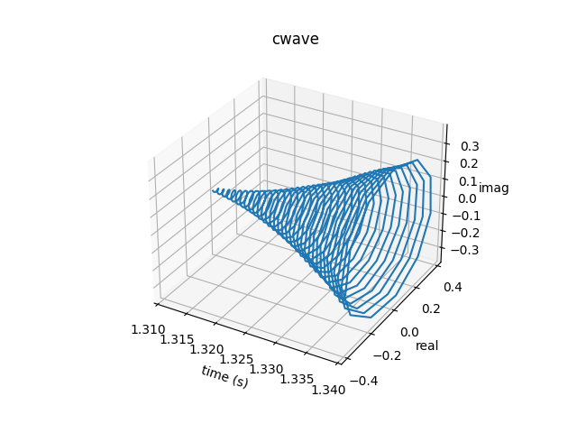
Viewing it as a complex waveform doesn’t really do us too much good, so let’s look at the real projection in 2D:

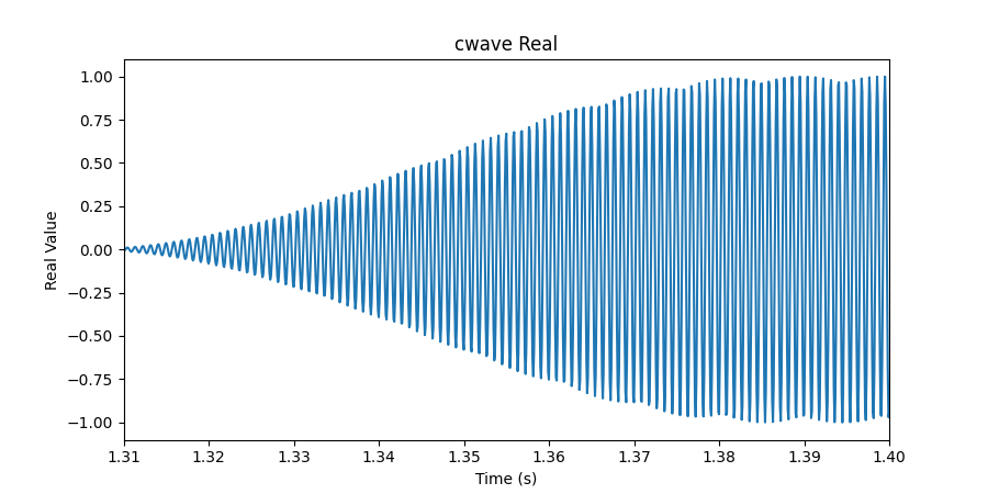
Now we’re getting somewhere. You can see the Gaussian-smoothed pulses (bumps that show up when the signal increases). You’d really have to zoom in and count to actually note the minor differences in frequency, but detecting those would be no trouble for an FFT.

Remember, this waveform looks perfect because it is! We’ve already decoded this signal and this a reconstruction. Next we’ll take a look at the actual radio data that was captured.

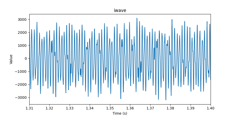
This is the actual sampled RF data stored in a two byte signed integer array shown in the time domain. As you can see, it’s pretty hard for the human eye to make heads or tails of it. dopspread scales iwave down to +/- 1 and multiplies it by the complex conjugate of cwave to get g, the estimated channel gain data:

g doesn’t help us much in the time domain, but in the frequency domain we can do a whole lot more. A complex to complex FFT with twice as many points as the samples in iwave and we get this:

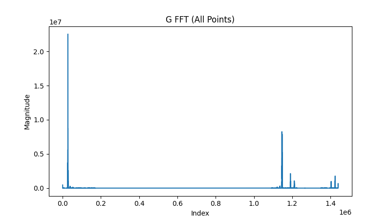
This is the only FFT the algorithm performs. It’s the basis for much of the analysis that follows and it’s important to note a few things:

The FFT can be broken down into two main regions, the power region, -1 Hz to 1 Hz, and the noise region, -4 Hz to 2 Hz and 2 Hz to 4 Hz. The analysis only takes place from -4 Hz to 4 Hz, but it appears -10 Hz to 10 Hz can be stored in a separate file (perhaps it provides a prettier picture?).

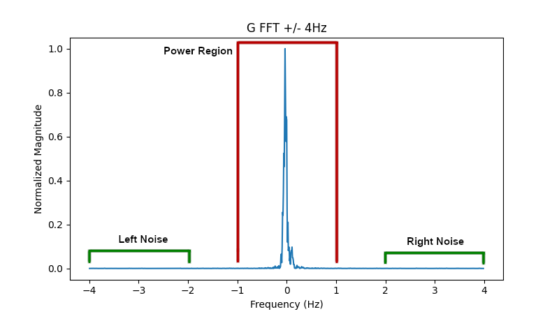
It starts by looking in the power region for the maximum signal (as calculated as the sum of the squares of the real and imaginary components of the signal). This is stored as smax which is used to scale the whole FFT down between the values of 0 and 1.

In the noise regions an average signal on each side is calculated. The minimum value of the two regions is then subtracted from the FFT, effectively removing any offset above zero.

Pay close attention to how the loops check to see if i is negative and set j accordingly:

For a negative i the FFT is actually indexed from the right hand side. Just visualizing the array without centering it will yield confusing results!

To fully understand the next part of the algorithm, it helps to pay close attention to the name of the variable it returns: w50. A bit of googling yields this paper in which Joe Taylor defines w50

The total power for the power region is stored in sum1. The Fortran code loops through the power region again, this time summing up the power as it goes and storing the index when it reaches 25 percent, 50 percent, and 75 percent in xi1, xi2, and xi3 respectively:

You may also notice the indexes it stores aren’t technically integers. It performs an overshoot correction of the form:

In this way if the percent power is somewhere between two indices, it can make a linear estimate as to where it would be and return a float.^[1]

The algorithm then takes the difference between the 75% power index and the 25% power index and attempts to prevent index differences less than one through the use of:

Graphing this shows how the minimum xdiff will be one:

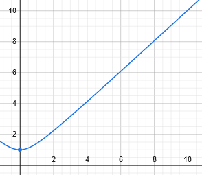
The difference in indexes is then converted to a difference in frequencies and voilà, you have the spread of frequencies over which half of the power of the transmission is contained: w50.

To summarize, here are the basic steps of the algorithm for FSTW4 Doppler spread calculations:

I’d be remiss if I didn’t check to see that my understanding was complete by implementing the algorithm myself. What follows is a Python implementation, using the same data (including the ideal generated waveform) as the Fortran implementation.

Running this gives me 0.051 for the Doppler spread, which is within 6% of the 0.054 the Fortran code gives.

You can find the Python implementation, the data used, the scripts used to make the plots, and my butchered fst4_decode.f90 in this repo. Hopefully with a greater understanding of how this algorithm works, it can be implemented for WSPR signals. If you don’t want to dive into the C code that makes up wsprd, it may even be possible to do it based on the c2 files that wsprdaemon already analyzes. The main difference would probably be in setting FOCUS_REGION, POWER_REGION, and NOISE_REGION.