Extended Network Growth in jr - Part 1

Goal

With the basics of the jr network established (see Introducing jr: A Peer-to-Peer Social Network), I wanted to simulate the growth of the extended network and find a mathematical model that describes this growth.

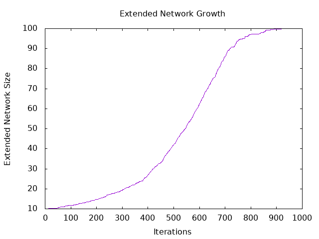
core/extended-network-test builds a test network of 100 nodes each following 10 random nodes. It then performs 1000 random syncs (two nodes chosen at random sync with each other) and records the average extended network size at each iteration. The output can be found in data/extended_growth.csv. Graphing the output with gnuplot¹ yields:

Fitting the Generalized Logistic Function

The graph appears to be a representation of the generalized logistic function which is fairly standard for systems that grow organically. The simplest form that fits our data is:

$$ Y(t) = A + \frac{K-A}{1+e^{-B(t-M)}} $$

Where $ A $ is the lower asymptote, $ K $ is the upper asymptote, $ B $ is the growth rate and $ M $ is the time at which the maximum growth rate occurs.

Using $ n $ for the total number of nodes and $ f $ for the number of nodes each node follows (as passed to sim/boostrap-network) $ A $ and $ K $ can be derived:

$$ A = f $$ $$ K = \min(n, f^2) $$

As a cost function I chose to use the sum of the squares of the residuals:

$$ ssr = \sum_{t=0}^{t=1000} (MeasuredValue[t] - Y(t))^2 $$

Where $ t $ is the number of random syncs that have been performed. This allows us to have a measure of how far off our guess of $ B $ and $ M $ is with the goal being to minimize the cost function. Since we are only dealing with two features we can create a 3D plot of the cost function using gradient/graph-ssr:

jr.core=> (gradient/graph-ssr 10 100 (gradient/read-csv "data/extended_growth.csv" 1))

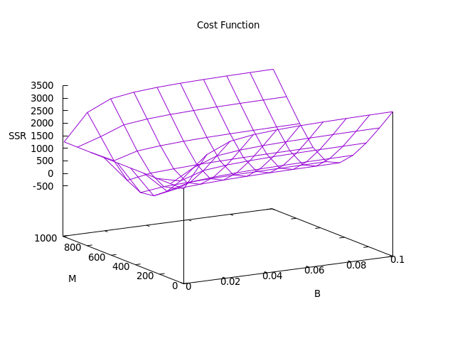
As we can see from the graph, the minimum occurs around $ B = 0.01 $ and $ M = 500 $. Using gradient descent, we will attempt to hone in on more precise values².

Fortunately the partial derivatives are already worked out in the Wikipedia article. All we need to do is update them for our simplified sigmoid:

$$ \frac{\partial{Y}}{\partial{B}} = \frac{(K-A)(t-M)e^{-B(t-M)}}{(1+e^{-B(t-M)})^2} $$ $$ \frac{\partial{Y}}{\partial{M}} = -\frac{(K-A)Be^{-B(t-M)}}{(1+e^{-B(t-M)})^2} $$

Some great examples of taking partial derivatives of a least squares function can be found here and here. The partial derivatives of our cost function with respect to $ B $ and $ M $ would be:

$$ \frac{\partial{ssr}}{\partial{B}} = -2\sum_{n=0}^{1000}\frac{\partial{Y}}{\partial{B}} * ssr $$ $$ \frac{\partial{ssr}}{\partial{M}} = -2\sum_{n=0}^{1000}\frac{\partial{Y}}{\partial{M}} * ssr $$

The functions for the partial derivatives as well as for the gradient are gradient/pdb, gradient/pdm, and gradient/grad respectively³. gradient/descent-to will perform a gradient descent algorithm with an adaptive learning rate³ (taking iterations from an infinite, lazy sequence) until the cost function does not change by a certain threshold. The output for our example can be seen here:

jr.core=> (gradient/descent-to 10 100 0.01 500 (gradient/read-csv "data/extended_growth.csv" 1) 0.001)
[5.116888516074428 0.010599133609303186 518.1614846831767]

As we can see the value $ B = 0.01 $ and $ M = 518 $ yield a minimum $ SSR $ of 5.11. Now that we have the tools we can try to build our mathematical model.

Determining the Effects of Following List Size ($ f $) on Extended Network Growth

core/multi-extended-growth changes the amount of nodes each node in the network follows ($ f $), calculates the extended network growth, and writes the results to data/multi_extended_growth.csv. Plotting the data, we can see the effect on our logistic curve as we vary $ f $ from 10 to 90:

jr.core=> (multi-extended-growth (range 10 100 10))
nil

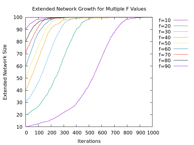
As we can see, increasing $ f $ appears to be shifting $ M $ to the left. This is exactly what we would expect as a greater :following list would mean a node achieves its maximum growth rate earlier.

To get a more precise model, we can also use our gradient descent implementation to calculate $ B $ and $ M $ for networks grown with differing values of $ f $. This is implemented in core/multi-descent. Unfortunately there aren’t a lot of values of $ f $ that we can work with. If we extend our range of $ t $ values to $ 3000 $ we can fit the curve down to $ f = 3 $. 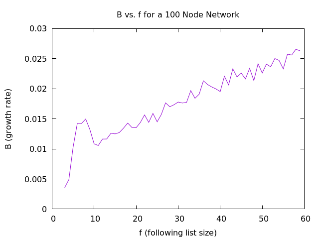The maximum $ f $ we can work with is around $ 60 $ if we still want to have enough of a curve to do a decent fit. Using core/multi-extended-growth and core/multi-descent we can create graphs for $ B $ and $ M $ as functions of $ f $:

jr.core=> (multi-extended-growth (range 3 60 1))
nil
jr.core=> (multi-descent (range 3 60 1))
nil

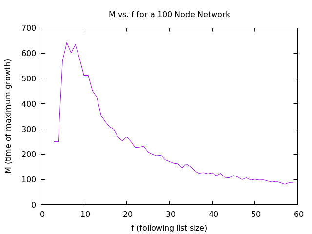
As can be seen, the first few points still do not get a good fit with the gradient descent method and the results are not great. The computation took several hours and I had to use an external tool to fit plots which is mildly annoying when you just spent a decent amount of time implementing a curve fitter. All that being said, for a network size of $ 100 $ the time of maximum growth, $ M $, can be predicted based on following list size, $ f $, with the following equation:

$$ M = \frac{5000}{f} $$

A rational function makes sense as one would expect it to be asymptotically bounded on each side. $ M $ should approach $ 0 $ as the following list, $ f $, increases and it should start at infinity for an impossible following list size of zero.

$ B $ does not appear to change that much as $ f $ varies, with only a slight linear upward trend with a slope of $ 0.0003 $.

If this conclusion seems underwhelming it’s because it is. Even as I write this I have partially implemented ideas for improvement. Before I expand this and see if that $ 5000 $ constant can be expressed in terms of $ n $ ($ \frac{n^2}{2} $ perhaps?) I’d like to tighten up the results. I’ve labeled this post Part 1 as I’m planning on taking a better look soon.

Functional Programming, Clojure, and Optimizing Gradient Descent

The purpose of this project is not only to learn more about gossip protocols as used by Secure Scuttlebutt, but also to learn more about functional programming and Clojure in particular. To that point, here are some reflections on going through the process in Clojure:

Visualizing Gradient Descent as an Infinite Sequence

It took a moment to realize that the results of gradient descent can be represented as an infinite sequence. It is so commonly thought of as a loop with a breaking condition that the mind-shift was difficult. I found looking at several implementations of the Fibonacci sequence in Clojure to be helpful in wrapping my head around it.

Optimizations in Functional Programming

Originally I was incorrectly under the assumption that results from a pure function (side effect free) were cached and if the parameters remained unchanged the cached results would be used. For example, if I repeatedly calculate the gradient of the same terms I expected a huge drop in the time the function took the second and third time. This is not the default, but it can be supported via memoization. Trying it out I began to run into issues with the overhead of calling functions. So much of what I was doing was simple math that may actually be less expensive than making a function call. What I ended using on was multi-arity functions where I pass the results of intensive calculations (gradient or $ e^{-B(T-M)} $) if I have them available. If not, they are calculated by the function.

Trending Towards Matrix Notation and Numerical Methods

Initially I wrote my partial derivative functions independently, gradient/pdb and gradient/pdm, but when I wrote my gradient function, gradient/grad, I returned a vector of results. In Clojure, it seems to make the most sense to work on everything as a vector more akin to matrix notation in mathematics. In fact if numerical methods are used⁴ these functions could easily work on arbitrary length vectors representing the parameters to a function that is passed as a parameter. Thus, Clojure seems to nudge you in the direction of creating a more general purpose gradient descent implementation and sometimes punishes you for being too specific. My gut tells me the generalized solution is the better way and if I were to do it again, I’d make it less specific.

Prior Work

Research does not occur in a vacuum and this project is no exception. There is an excellent thesis on message passing via gossip protocols by Mohsen Taghavianfar that can be found here. It has a fantastic quote that I’d like to address:

Most investigations done in this field just assume that a logistic function is necessarily involved, however, according to the best of my knowledge none of them explain why we need such an assumption.⁵

In my case I started with the simulation, saw that the analysis was going to be complex (remember we’re simulating Secure Scuttlebutt meaning we have to simulate the friend-of-friend nature of message passing as well as the establishment of the friend-of-friend network), generated growth output for the first part of my problem (network establishment), and saw that it looked like a logistic. Due to the complexity, I did not attempt to attack this analytically at first.

Taghavianfar does a great job reviewing previous work and he includes all of the code for the simulation as well as the output. The references in the paper are a great source for further exploration as well. I highly recommend reading this work.